Joining data

Code for Quiz 6, more dplyr and our first interactive chart using echarts4r

Steps 1-6

1. Load the R packages we will use

library(tidyverse)
library(echarts4r)
library(hrbrthemes)

2. Read the data in the file, drug_cos.csv, health_cos.csv in to R and assign to the variables drug_cos and health_cos, respectively

drug_cos <- read_csv("https://estanny.com/static/week6/drug_cos.csv")
health_cos <- read_csv("https://estanny.com/static/week6/health_cos.csv")

3. Use glimpse to get a glimpse of the data

drug_cos %>% glimpse()

Rows: 104
Columns: 9
$ ticker       <chr> "ZTS", "ZTS", "ZTS", "ZTS", "ZTS", "ZTS", "Z...
$ name         <chr> "Zoetis Inc", "Zoetis Inc", "Zoetis Inc", "Z...
$ location     <chr> "New Jersey; U.S.A", "New Jersey; U.S.A", "N...
$ ebitdamargin <dbl> 0.149, 0.217, 0.222, 0.238, 0.182, 0.335, 0....
$ grossmargin  <dbl> 0.610, 0.640, 0.634, 0.641, 0.635, 0.659, 0....
$ netmargin    <dbl> 0.058, 0.101, 0.111, 0.122, 0.071, 0.168, 0....
$ ros          <dbl> 0.101, 0.171, 0.176, 0.195, 0.140, 0.286, 0....
$ roe          <dbl> 0.069, 0.113, 0.612, 0.465, 0.285, 0.587, 0....
$ year         <dbl> 2011, 2012, 2013, 2014, 2015, 2016, 2017, 20...

health_cos %>% glimpse()

Rows: 464
Columns: 11
$ ticker      <chr> "ZTS", "ZTS", "ZTS", "ZTS", "ZTS", "ZTS", "ZT...
$ name        <chr> "Zoetis Inc", "Zoetis Inc", "Zoetis Inc", "Zo...
$ revenue     <dbl> 4233000000, 4336000000, 4561000000, 478500000...
$ gp          <dbl> 2581000000, 2773000000, 2892000000, 306800000...
$ rnd         <dbl> 427000000, 409000000, 399000000, 396000000, 3...
$ netincome   <dbl> 245000000, 436000000, 504000000, 583000000, 3...
$ assets      <dbl> 5711000000, 6262000000, 6558000000, 658800000...
$ liabilities <dbl> 1975000000, 2221000000, 5596000000, 525100000...
$ marketcap   <dbl> NA, NA, 16345223371, 21572007994, 23860348635...
$ year        <dbl> 2011, 2012, 2013, 2014, 2015, 2016, 2017, 201...
$ industry    <chr> "Drug Manufacturers - Specialty & Generic", "...

4. Which variables are the same in both data sets

names_drug <- drug_cos %>% names()
names_health <- health_cos %>% names()
intersect(names_drug, names_health)

[1] "ticker" "name"   "year"  

5. Select subset of variables to work with

• For drug_cos select (in this order): ticker, year, grossmargin

  • Extract observations for 2018

  • Assign output to drug_subset

• For health_cos select (in this order): ticker, year, revenue, gp, industry

  • Extract observations for 2018

  • Assign output to health_subset

drug_subset <- drug_cos %>%
  select(ticker, year, grossmargin) %>%
  filter(year == 2018)
health_subset <- health_cos %>%
  select(ticker, year, revenue, gp, industry)%>%
  filter(year == 2018)

6. Keep all the rows and columns drug_select join with columns in health_subset

drug_subset %>% left_join(health_subset)

# A tibble: 13 x 6
   ticker  year grossmargin   revenue        gp industry              
   <chr>  <dbl>       <dbl>     <dbl>     <dbl> <chr>                 
 1 ZTS     2018       0.672   5.82e 9   3.91e 9 Drug Manufacturers - ~
 2 PRGO    2018       0.387   4.73e 9   1.83e 9 Drug Manufacturers - ~
 3 PFE     2018       0.79    5.36e10   4.24e10 Drug Manufacturers - ~
 4 MYL     2018       0.35    1.14e10   4.00e 9 Drug Manufacturers - ~
 5 MRK     2018       0.681   4.23e10   2.88e10 Drug Manufacturers - ~
 6 LLY     2018       0.738   2.46e10   1.81e10 Drug Manufacturers - ~
 7 JNJ     2018       0.668   8.16e10   5.45e10 Drug Manufacturers - ~
 8 GILD    2018       0.781   2.21e10   1.73e10 Drug Manufacturers - ~
 9 BMY     2018       0.71    2.26e10   1.60e10 Drug Manufacturers - ~
10 BIIB    2018       0.865   1.35e10   1.16e10 Drug Manufacturers - ~
11 AMGN    2018       0.827   2.37e10   1.96e10 Drug Manufacturers - ~
12 AGN     2018       0.861   1.58e10   1.36e10 Drug Manufacturers - ~
13 ABBV    2018       0.764   3.28e10   2.50e10 Drug Manufacturers - ~

Questions: join_ticker

• Start with drug_cos

• Extract observations for the ticker MRK from drug_cos

• Assign output to the variable drug_cos_subset

drug_cos_subset <- drug_cos %>%
  filter(ticker == "MRK")

---

• Display drug_cos_subset

drug_cos_subset

# A tibble: 8 x 9
  ticker name  location ebitdamargin grossmargin netmargin   ros   roe
  <chr>  <chr> <chr>           <dbl>       <dbl>     <dbl> <dbl> <dbl>
1 MRK    Merc~ New Jer~        0.305       0.649     0.131 0.15  0.114
2 MRK    Merc~ New Jer~        0.33        0.652     0.13  0.182 0.113
3 MRK    Merc~ New Jer~        0.282       0.615     0.1   0.123 0.089
4 MRK    Merc~ New Jer~        0.567       0.603     0.282 0.409 0.248
5 MRK    Merc~ New Jer~        0.298       0.622     0.112 0.136 0.096
6 MRK    Merc~ New Jer~        0.254       0.648     0.098 0.117 0.092
7 MRK    Merc~ New Jer~        0.278       0.678     0.06  0.162 0.063
8 MRK    Merc~ New Jer~        0.313       0.681     0.147 0.206 0.199
# ... with 1 more variable: year <dbl>

• Use left_join to combine the rows and columns of drug_cos_subset with the columns of health_cos

• Assign the output to combo_df

combo_df <- drug_cos_subset %>%
  left_join(health_cos)

---

• Display combo_df

combo_df

# A tibble: 8 x 17
  ticker name  location ebitdamargin grossmargin netmargin   ros   roe
  <chr>  <chr> <chr>           <dbl>       <dbl>     <dbl> <dbl> <dbl>
1 MRK    Merc~ New Jer~        0.305       0.649     0.131 0.15  0.114
2 MRK    Merc~ New Jer~        0.33        0.652     0.13  0.182 0.113
3 MRK    Merc~ New Jer~        0.282       0.615     0.1   0.123 0.089
4 MRK    Merc~ New Jer~        0.567       0.603     0.282 0.409 0.248
5 MRK    Merc~ New Jer~        0.298       0.622     0.112 0.136 0.096
6 MRK    Merc~ New Jer~        0.254       0.648     0.098 0.117 0.092
7 MRK    Merc~ New Jer~        0.278       0.678     0.06  0.162 0.063
8 MRK    Merc~ New Jer~        0.313       0.681     0.147 0.206 0.199
# ... with 9 more variables: year <dbl>, revenue <dbl>, gp <dbl>,
#   rnd <dbl>, netincome <dbl>, assets <dbl>, liabilities <dbl>,
#   marketcap <dbl>, industry <chr>

• Note: the variables ticker, name, location, and industry are the same for all the observations

---

• Assign the company name to co_name

co_name <- combo_df %>%
  distinct(name)%>%
  pull()

---

• Assign the company location to co_location

co_location <- combo_df %>%
  distinct(location)%>%
  pull()

---

• Assign the industry to co_indsutry group

co_industry <- combo_df %>%
  distinct(industry)%>%
  pull()

Pu the r inline commands used in the blanks below. When you knit the document the results of the commands will be displayed in your text.

The company ??? is located in ??? and is a member of the ??? industry group

---

• Start with combo_df

• Select variables (in this order): year, grossmargin, netmargin, revenue, gp, netincome

• Assign the output to combo_df_subset

combo_df_subset <- combo_df %>%
  select(year, grossmargin, netmargin,
         revenue, gp, netincome)

---

• Display combo_df_subset

combo_df_subset

# A tibble: 8 x 6
   year grossmargin netmargin     revenue          gp   netincome
  <dbl>       <dbl>     <dbl>       <dbl>       <dbl>       <dbl>
1  2011       0.649     0.131 48047000000 31176000000  6272000000
2  2012       0.652     0.13  47267000000 30821000000  6168000000
3  2013       0.615     0.1   44033000000 27079000000  4404000000
4  2014       0.603     0.282 42237000000 25469000000 11920000000
5  2015       0.622     0.112 39498000000 24564000000  4442000000
6  2016       0.648     0.098 39807000000 25777000000  3920000000
7  2017       0.678     0.06  40122000000 27210000000  2394000000
8  2018       0.681     0.147 42294000000 28785000000  6220000000

---

• Create the variable grossmarign_check to compare with the variable grossmargin. They should be equal.
  • grossmargin_check = gp / revenue
• Create the variable close_margin to check that the absolute value of the difference between grossmargin_check and grossmargin is less than 0.001

combo_df_subset %>%
  mutate(grossmargin_check = gp / revenue,
  close_margin = abs(grossmargin_check - grossmargin) < 0.001)

# A tibble: 8 x 8
   year grossmargin netmargin revenue      gp netincome
  <dbl>       <dbl>     <dbl>   <dbl>   <dbl>     <dbl>
1  2011       0.649     0.131 4.80e10 3.12e10   6.27e 9
2  2012       0.652     0.13  4.73e10 3.08e10   6.17e 9
3  2013       0.615     0.1   4.40e10 2.71e10   4.40e 9
4  2014       0.603     0.282 4.22e10 2.55e10   1.19e10
5  2015       0.622     0.112 3.95e10 2.46e10   4.44e 9
6  2016       0.648     0.098 3.98e10 2.58e10   3.92e 9
7  2017       0.678     0.06  4.01e10 2.72e10   2.39e 9
8  2018       0.681     0.147 4.23e10 2.88e10   6.22e 9
# ... with 2 more variables: grossmargin_check <dbl>,
#   close_margin <lgl>

---

• Create the variable netmargin_check to compare witht he variable netmargin. They should be equal.

• Create the variable close_enough to check that the absolute value of the difference between netmargin_check and netmargin is less than 0.001

combo_df_subset %>%
  mutate(netmargin_check = netincome / revenue,
      close_enough = abs(netmargin_check - netmargin) < 0.001)

# A tibble: 8 x 8
   year grossmargin netmargin revenue      gp netincome
  <dbl>       <dbl>     <dbl>   <dbl>   <dbl>     <dbl>
1  2011       0.649     0.131 4.80e10 3.12e10   6.27e 9
2  2012       0.652     0.13  4.73e10 3.08e10   6.17e 9
3  2013       0.615     0.1   4.40e10 2.71e10   4.40e 9
4  2014       0.603     0.282 4.22e10 2.55e10   1.19e10
5  2015       0.622     0.112 3.95e10 2.46e10   4.44e 9
6  2016       0.648     0.098 3.98e10 2.58e10   3.92e 9
7  2017       0.678     0.06  4.01e10 2.72e10   2.39e 9
8  2018       0.681     0.147 4.23e10 2.88e10   6.22e 9
# ... with 2 more variables: netmargin_check <dbl>,
#   close_enough <lgl>

Question: summarize_industry

• Fill in the blanks

• Put the command you use in the Rchunks in the Rmd file for this quiz

• Use the health_cos data

• For each industry calculate

  • mean_netmargin_percent = mean(netincome / revenue) * 100
  • median_netmargin_percent = median(netincome / revenue) * 100
  • min_netmargin_percent = min(netincome / revenue) * 100
  • max_netmargin_percent = max(netincome / revenue) * 100

health_cos %>%
  group_by(industry) %>%
  summarize(mean_netmargin_percent = mean(netincome / revenue)*100,
            median_netmargin_percent = median(netincome / revenue)*100,
            min_netmargin_percent = min(netincome / revenue)*100,
            max_netmargin_percent = max(netincome / revenue)*100)

# A tibble: 9 x 5
  industry mean_netmargin_~ median_netmargi~ min_netmargin_p~
* <chr>               <dbl>            <dbl>            <dbl>
1 Biotech~            -4.66             7.62         -197.   
2 Diagnos~            13.1             12.3             0.399
3 Drug Ma~            19.4             19.5           -34.9  
4 Drug Ma~             5.88             9.01          -76.0  
5 Healthc~             3.28             3.37           -0.305
6 Medical~             6.10             6.46            1.40 
7 Medical~            12.4             14.3           -56.1  
8 Medical~             1.70             1.03           -0.102
9 Medical~            12.3             14.0           -47.1  
# ... with 1 more variable: max_netmargin_percent <dbl>

• mean_netmargin_percent for the industry Diagnostics & Research is 13.1%
• median_netmargin_percent for the industry Diagnostics & Research is 12.3%
• min_netmargin_percent for the industry Diagnostics & Research is 0.399%
• max_netmargin_percent for the industry Diagnostics & Research is 26.3%

Question: inline_ticker

• Fill in the blanks

• Use the health_cos data

• Extract observations for the ticker AMGN from health_cos and assign to the variable health_cos_subset

health_cos_subset <- health_cos %>%
  filter(ticker == "AMGN")

• Display health_cos_subset

health_cos_subset

# A tibble: 8 x 11
  ticker name  revenue      gp    rnd netincome  assets liabilities
  <chr>  <chr>   <dbl>   <dbl>  <dbl>     <dbl>   <dbl>       <dbl>
1 AMGN   Amge~ 1.56e10 1.29e10 3.17e9    3.68e9 4.89e10 29842000000
2 AMGN   Amge~ 1.73e10 1.41e10 3.38e9    4.34e9 5.43e10 35238000000
3 AMGN   Amge~ 1.87e10 1.53e10 4.08e9    5.08e9 6.61e10 44029000000
4 AMGN   Amge~ 2.01e10 1.56e10 4.30e9    5.16e9 6.90e10 43231000000
5 AMGN   Amge~ 2.17e10 1.74e10 4.07e9    6.94e9 7.14e10 43366000000
6 AMGN   Amge~ 2.30e10 1.88e10 3.84e9    7.72e9 7.76e10 47751000000
7 AMGN   Amge~ 2.28e10 1.88e10 3.56e9    1.98e9 8.00e10 54713000000
8 AMGN   Amge~ 2.37e10 1.96e10 3.74e9    8.39e9 6.64e10 53916000000
# ... with 3 more variables: marketcap <dbl>, year <dbl>,
#   industry <chr>

• In the console, type ?distinct. Go to the help pane to see what distinct does
• In the console, type ?pull. GO to the help pane to see hat pull does

Run the code below

health_cos_subset %>%
  distinct(name)%>%
  pull(name)

[1] "Amgen Inc"

• Assign the output to co_name

co_name <- health_cos_subset %>%
  distinct(name)%>%
  pull(name)

You can take output from your code and include it in your text.

• The name of the company with ticker AMGN is Amgen Inc in following chunk

• Assign the company’s industry group to the variable co_industry

co_industry <- health_cos_subset %>%
  distinct(industry) %>%
  pull()

THis is outside the Rchunk. Put the r inline commands used in the blanks below. When you knit the document the results of the commands will be displayed in your text.

The company Amgen Inc is a member of the Drug Manufacturers - General group.

Steps 7-11

7. Prepare the data for the plots

• start with health_cos THEN
• group_by industry THEN
• calculate the median research and development expenditure by industry
• assign the output to df

df <- health_cos %>%
  group_by(industry) %>%
  summarize(med_rnd_rev = median(rnd/revenue))

8. Use glimpse to glimpse the data for the plots

df %>% glimpse()

Rows: 9
Columns: 2
$ industry    <chr> "Biotechnology", "Diagnostics & Research", "D...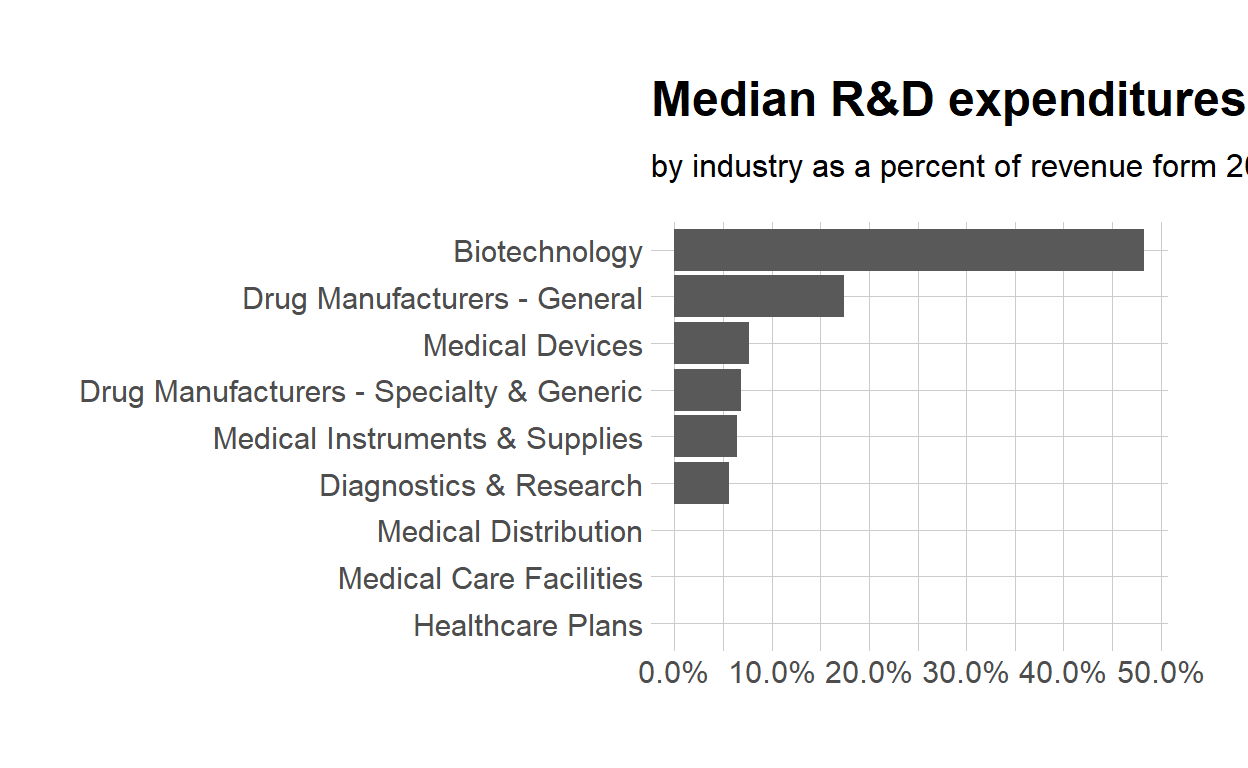
$ med_rnd_rev <dbl> 0.48317287, 0.05620271, 0.17451442, 0.0685187...

9. Create a static bar chart

• use ggplot to initialize the chart
• data is df
• the variable industry is mapped to the x-axis
  • reorder it based the value of med_rnd_rev
• the variable med_rnd_rev is mapped to the y-axis
• add a bar chart using geom_col
• use scale_y_continuous to label the y-axis with percent
• use coord_flip() to flip the coordinates
• use labs to add title, subtitle and remove x and y-axes
• use theme_ipsum() from the hrbthemes package to improve the theme

ggplot(data = df, mapping = aes(
  x = reorder(industry, med_rnd_rev),
  y = med_rnd_rev
  ))+
  geom_col()+
  scale_y_continuous(labels = scales::percent)+
  coord_flip()+
  labs(
    title = "Median R&D expenditures",
    subtitle = "by industry as a percent of revenue form 2011 to 2018",
    x = NULL, y = NULL)+
  theme_ipsum()

10. Save the last plot to preview.png and add to the yaml chunk at the top

ggsave(filename = "preview.png",
       path = here::here("_posts", "2021-03-11-joining-data"))

11. Create an interactive bar char using the package echarts4r

• start with the data df
• use arrange to reorder med_rnd_rev
• use e_charts to initialize chart
  • the variable industry is mapped to the x-axis
• add a bar chart using e_bar with the value of med_rnd_rev
• use e_flip_coords() to flip the coordinates
• use e_title to add the title and the subtitle
• use e_legend to remove the legends
• use e_x_axis to change the format of the labels on x-axis to percent
• use e_y_axis to remove labels on y-axis
• use e_theme to change the theme. Find more themes here

df %>%
  arrange(med_rnd_rev) %>%
  e_charts(
    x = industry
  ) %>%
  e_bar(
    serie = med_rnd_rev,
    name = "medium"
  ) %>%
  e_flip_coords() %>%
  e_tooltip() %>%
  e_title(
    text = "Median industry R&D expenditures",
    subtext = "by industry as a percent of evenue from 2011 to 2018",
    left = "center") %>%
  e_legend(FALSE) %>%
  e_x_axis(
    formatter = e_axis_formatter("percent", digits = 0)
  ) %>%
  e_y_axis(
    show = FALSE
  ) %>%
  e_theme("infogrpahic")